4. Tips and tricks

4.1. Fonts

No font information in the DOT file is preserved by dot2tex. However, there are several ways of modifying the generated LaTeX code to achieve some control of fonts and font sizes.

• Modifying the templates.
• Using the d2tdocpreamble and d2tfigpreamble attributes or command line options.
• Using the lblstyle attribute.

To increase the font size you can for instance insert a \Huge command in the figure preamble:

$ dot2tex -tmath --figpreamble="\Huge" ex1.dot > ex1huge.tex

4.2. Debugging

When making your own templates it is easy to make mistakes, and LaTeX markup in graphs may fail to compile. To make it easier to find errors, invoke dot2tex with the --debug option:

$ dot2tex --preproc --debug test.dot

A dot2tex.log file will then be generated with detailed information. In the log file you will find the generated LaTeX code, as well as well as the compilation log.

4.3. Be consistent

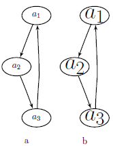
Be aware of differences between the template you use for preprocessing and code used to generate final output. This is especially important if you use the --figonly option and include the code in a master document. If a 10pt font is used during preprocessing, the result may not be optimal if a 12pt font is used in the final output.

Example. A graph is generated with:

$ dot2tex --preproc -tmath --nominsize ex1.dot > ex1tmp.dot

Running through dot2tex again with:

$ dot2tex --figpreamble="\Huge" ex1tmp.dot > ex1huge.tex

gives labels that do not fit properly inside the nodes.

4.4. Postprocessing

The output from Graphviz and dot2tex is not perfect. Manual adjustments are sometimes necessary to get the right results for use in a publication. For final and cosmetic adjustments, it is often easier to edit the generated code than to hack the dot source. This is especially true when using the tikz output format.

4.5. Use the special graph attributes

Dot2tex has many options for customizing the output. Sometimes is is impractical or boring to type the various options at the command line each time you want to create the graph. To avoid this, you can use the special graph attributes. The d2toptions attribute is handy because it is interpreted as command line options.

So instead of typing:

$ dot2tex -tikz -tmath --tikzedgelabels ex1.dot

each time, use d2toptions like this:

digraph G {
    d2toptions ="-tikz -tmath --tikzedgelabels";
    ...
}

4.6. Use the tikz output format for maximum flexibility

The difference between the pgf and tikz output formats is best shown with an example. Consider the following graph:

graph G {
    mindist = 0.5;
    node [shape=circle];
    a -- b -- c -- a;
}

Rendering the graph using circo and the pgf and tikz output formats:

$ circo -Txdot simple.dot | dot2tex -tmath -fpgf -s
$ circo -Txdot simple.dot | dot2tex -tmath -ftikz -s

gives visually different graphs:

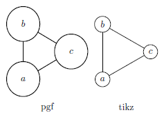
However, the main difference is in the generated code. Here is the pgf output:

% Edge: a -- b
\draw [] (19bp,38bp) -- (19bp,60bp);
% Edge: b -- c
\draw [] (35bp,70bp) -- (55bp,58bp);
% Edge: c -- a
\draw [] (55bp,40bp) -- (35bp,28bp);
% Node: a
\begin{scope}
\pgfsetstrokecolor{black}
\draw (19bp,19bp) ellipse (18bp and 19bp);
\draw (19bp,19bp) node {$a$};
\end{scope}
% Node: b
\begin{scope}
\pgfsetstrokecolor{black}
\draw (19bp,79bp) ellipse (18bp and 19bp);
\draw (19bp,79bp) node {$b$};
\end{scope}
% Node: c
\begin{scope}
\pgfsetstrokecolor{black}
\draw (71bp,49bp) ellipse (18bp and 19bp);
\draw (71bp,49bp) node {$c$};
\end{scope}

Compare the above code with the tikz output:

\node (a) at (19bp,19bp) [draw,circle,] {$a$};
\node (b) at (19bp,79bp) [draw,circle,] {$b$};
\node (c) at (71bp,49bp) [draw,circle,] {$c$};
\draw [] (a) -- (b);
\draw [] (b) -- (c);
\draw [] (c) -- (a);

The code is much more compact and it is quite easy to modify the graph.

4.7. The dot2texi LaTeX package

The dot2texi package allows you to embed DOT graphs directly in you LaTeX document. The package will automatically run dot2tex for you and include the generated code. Example:

\documentclass{article}
\usepackage{dot2texi}

\usepackage{tikz}
\usetikzlibrary{shapes,arrows}

\begin{document}
\begin{dot2tex}[neato,options=-tmath]
digraph G {
    node [shape="circle"];
    a_1 -> a_2 -> a_3 -> a_4 -> a_1;
    }
\end{dot2tex}

\end{document}

When the above code is run through LaTeX, the following will happen is shell escape is enabled:

• The graph is written to file.
• dot2tex is run on the DOT file.
• The generated code is included in the document.

The whole process is completely automated. The generated graph will look like this:

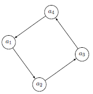
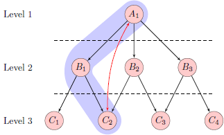
The codeonly option is useful in conjunction with dot2texi, especially when used with the tikz output format. Here is an example that shows how to annotate a graph:

\documentclass{article}
\usepackage{tikz}
\usetikzlibrary{arrows,shapes}
\usepackage{dot2texi}
\begin{document}
% Define layers
\pgfdeclarelayer{background}
\pgfdeclarelayer{foreground}
\pgfsetlayers{background,main,foreground}

% The scale option is useful for adjusting spacing between nodes.
% Note that this works best when straight lines are used to connect
% the nodes.
\begin{tikzpicture}[>=latex',scale=0.8]
    % set node style
    \tikzstyle{n} = [draw,shape=circle,minimum size=2em,
                        inner sep=0pt,fill=red!20]
    \begin{dot2tex}[dot,tikz,codeonly,styleonly,options=-s -tmath]
        digraph G  {
            node [style="n"];
            A_1 -> B_1; A_1 -> B_2; A_1 -> B_3;
            B_1 -> C_1; B_1 -> C_2;
            B_2 -> C_2; B_2 -> C_3;
            B_3 -> C_3; B_3 -> C_4;
        }
    \end{dot2tex}
    % annotations
    \node[left=1em] at (C_1.west)  (l3) {Level 3};
    \node at (l3 |- B_1) (l2){Level 2};
    \node at (l3 |- A_1) (l1) {Level 1};
    % Draw lines to separate the levels. First we need to calculate
    % where the middle is.
    \path (l3) -- coordinate (l32) (l2) -- coordinate (l21) (l1);
    \draw[dashed] (C_1 |- l32) -- (l32 -| C_4);
    \draw[dashed] (C_1 |- l21) -- (l21 -| C_4);
    \draw[<->,red] (A_1) to[out=-120,in=90] (C_2);
    % Highlight the A_1 -> B_1 -> C_2 path. Use layers to draw
    % behind everything.
    \begin{pgfonlayer}{background}
        \draw[rounded corners=2em,line width=3em,blue!20,cap=round]
                (A_1.center) -- (B_1.west) -- (C_2.center);
    \end{pgfonlayer}
\end{tikzpicture}
\end{document}

Note

If you don’t want to include the dot directly in your document, you can use the \input{..} command. See the section Including external dot files for more details.